Usage Guide
This guide covers how to install, configure, and use LevSeq-Dash for visualizing and analyzing directed evolution experiments.
Installation
Prerequisites
Python 3.9 or higher
Docker (optional, for containerized deployment)
Git
Quick Start with Docker
The fastest way to get started is using Docker:
# Clone the repository
git clone https://github.com/ssec-jhu/levseq-dash.git
cd levseq-dash

# Build the Docker image
docker build . -t levseq-dash:latest --no-cache

# Run in Public Playground mode
docker run -p 8050:8050 levseq-dash:latest
The application will be available at http://0.0.0.0:8050
Local Installation
For development or local use without Docker:
# Clone the repository
git clone https://github.com/ssec-jhu/levseq-dash.git
cd levseq-dash

# Install dependencies
pip install -r requirements/requirements.txt

# Run the application
python -m levseq_dash.app.main_app
Configuration
Deployment Modes
LevSeq-Dash supports two deployment modes:
Public Playground Mode
This mode is the fastest way to run the app and is ideal for demos, testing, and exploration of the curated sample dataset publicly available online at https://enzengdb.org/
Read-only mode with example data
No data modification allowed
Perfect for exploring features and testing
Uses pre-loaded sample experiments
Local Instance Mode
Use this mode for setting up an instance in your lab with persistent, user-controlled data storage.
Full read/write access for lab use
Upload and manage your own experiments
Delete experiments as needed
Customize data storage location
Set unique experiment ID prefixes for your lab
Local Instance Setup
Step 1: Configure config.yaml
Open levseq_dash/app/config/config.yaml and configure it for local instance mode.
💡 Hint: You can copy/paste the configuration below and modify the values:
# Set deployment mode to local-instance
deployment-mode: "local-instance"

disk:
  # Enable data modification to allow adding/deleting data
  enable-data-modification: true

  # Set a unique 5-letter prefix for your lab or project
  # OR set using environment variable
  five-letter-id-prefix: "MYLAB"

  # Example: absolute path of data on your desktop
  local-data-path: "/Users/<username>/Desktop/MyLabData"
Step 2: Configure five-letter-id-prefix
This should be a unique identifier for your lab or project (e.g., “MYLAB”, “JONES”)
It must be exactly 5 letters long and can only contain alphabetic characters (A-Z, a-z)
This will be prefixed to all your experiment IDs (e.g., “MYLAB-EXP001”)
Helps distinguish experiments from different labs/projects
Step 3: Configure local-data-path
This is where your experiment data will be stored on your local machine
Use an absolute path (e.g.,
/Users/username/Desktop/MyLabData)Make sure the directory exists and that you have write permissions to it
All uploaded experiments will be stored here
Using Docker with Environment Variables
You can override config.yaml settings at runtime using environment variables to set up multiple instances:
FIVE_LETTER_ID_PREFIX: Configure the 5-letter prefixDATA_PATH: Configure the local data path
Docker Run Example:
# Run in local instance mode using settings in config.yaml
docker run -p 8050:8050 levseq-dash:local

# OR run with environment variables to override config.yaml settings
docker run -p 8050:8050 \
    -v /your/host/data/path:/data \
    -e DATA_PATH=/data \
    -e FIVE_LETTER_ID_PREFIX=MYLAB \
    levseq-dash:local
Parameters Explained:
-v /your/host/data/path:/data: Mounts a directory from your host machine to the/datadirectory inside the container-e DATA_PATH=/data: Tells the application to use the/datadirectory for storage-e FIVE_LETTER_ID_PREFIX=MYLAB: Sets your unique 5-letter lab/project identifier
Logging and Debugging
Enable detailed logging for development and debugging:
# Logging and profiling settings for development and debugging
logging:
  # Enable profiling for sequence alignment performance testing
  # Logs timing information for alignment operations (default: false)
  sequence-alignment-profiling: true

  # Enable detailed logging for data manager operations
  # Logs data loading, experiment management operations (default: false)
  data-manager: true

  # Enable logging for pairwise aligner detailed operations
  # Logs alignment algorithm details and performance (default: false)
  pairwise-aligner: true
Logging Parameters:
sequence-alignment-profiling: Enables timing logs for sequence alignment operations, useful for performance optimizationdata-manager: Enables detailed logging of data loading, experiment metadata operations, and file I/Opairwise-aligner: Enables verbose logging of the BioPython pairwise alignment algorithm details
Note
These logging settings are primarily for development and debugging. Set all to false in production deployments to reduce log verbosity.
Uploading Experiments
Navigate to the Upload page
Prepare your data:
CSV file: Experiment data with required columns (see below)
CIF file: Protein structure file in cif file (PDB format is not yet supported)
Fill in the metadata form:
Lab Experiment ID
Parent Sequence
Experiment Description
Date of the experiment
Valid SMILES strings used in the experiment as substrate and product
Click Upload to validate and store the experiment
On success, you will see a confirmation message and can navigate to the experiment page.
If there are errors, they will be displayed for correction.
Required CSV Columns
Your CSV file must include these columns:
smiles_string: Chemical structure in SMILES formatfitness_value: Activity/fitness measurementwell: Well position (e.g., “A01”, “B12”) - must be in standard 96-well plate format (A1-H12)plate: Plate identifier (e.g., “1”, “2”, “Plate1”)amino_acid_substitutions: Amino acid mutations (e.g., “A123G”, “M45K”)Must include at least one row with
#PARENT#as the value to represent the parent sequence
alignment_count: Number of sequence alignmentsalignment_probability: Probability score for the alignment
Note
All SMILES strings must be valid chemical structures. Invalid SMILES will cause upload to fail with an error message indicating which row contains the invalid SMILES.
Exploring The Database
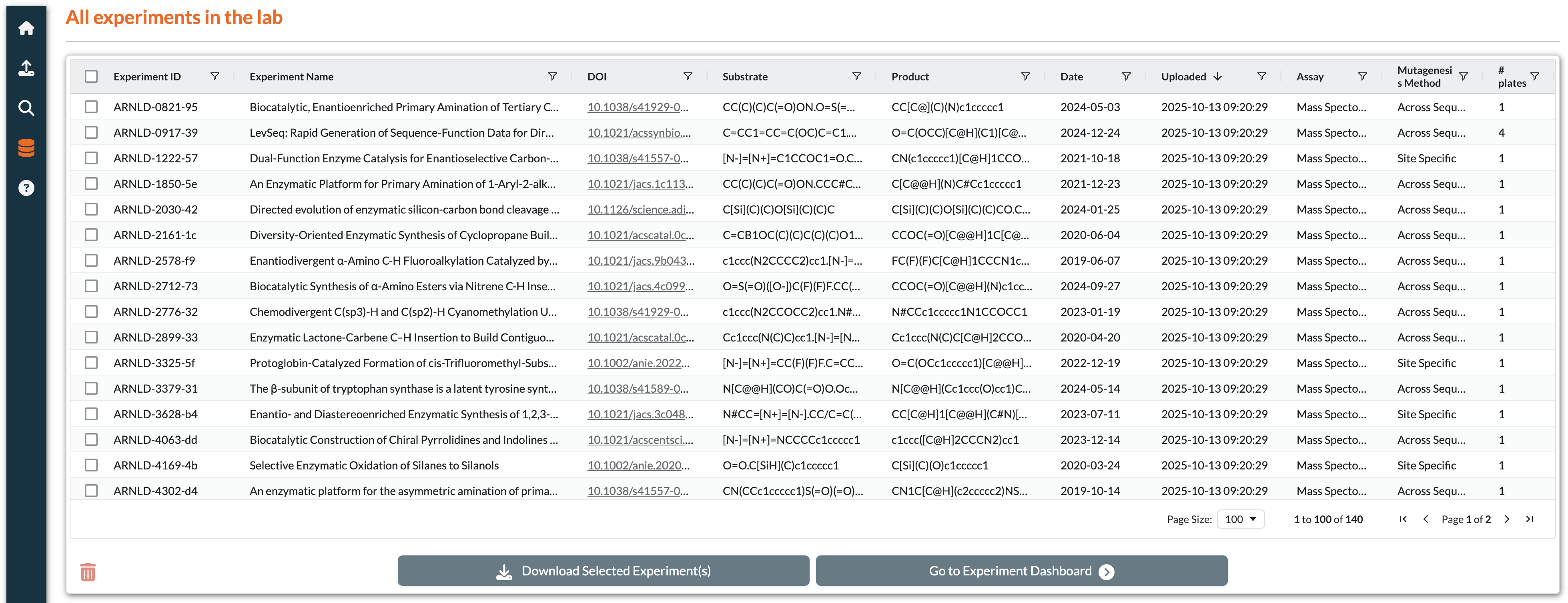
Explore page with experiment table, filters, and batch operation buttons
Features:
View table of all uploaded experiments with metadata
Interactive controls for filtering, sorting, and searching
Select experiments to perform batch operations
Export data in multiple formats
Table Interactions:
- Selection:
Single Selection: Click any row to select it
Multi-Selection: Hold Ctrl (Cmd on Mac) and click multiple rows
- Filtering and Sorting:
Column Filters: Click the filter icon in column headers to access filters
Text Search: Type in filter boxes to search within specific columns
Sorting: Click column headers to toggle ascending/descending sort
Filter Persistence: Filters are automatically saved in browser session storage
- Data Export:
Export Filtered Data: Download a CSV file containing only the currently filtered rows
Export Selected: Download multiple experiments as a ZIP file (see Actions below)
Available Actions (Buttons activate based on row selection):
Go To Experiment: Navigate to detailed experiment view
Requires: Exactly 1 row selected
Download Selected Experiments: Export experiments as a ZIP archive
Requires: 1 or more rows selected
Delete: Remove experiment from the system
Requires: Exactly 1 row selected
Only available in Local Instance mode
Note: Files are moved to a backup folder, not permanently deleted
Single Experiment Page
After selecting an experiment from the Explore page, you can view detailed analysis and visualizations.
Page Components:
Protein Structure Viewer: 3D visualization (if CIF file provided)
Experiment Metadata Panel: Shows experiment details
Top Variants Table: Interactive table of all variants
Heatmap: Visualizes variant data across well plates
Retention of Function Curve / Site Specific Plot: Shows variant rankings by fitness
Reaction Visualization: Displays substrate/product chemistry
Protein Structure Viewer (3D)
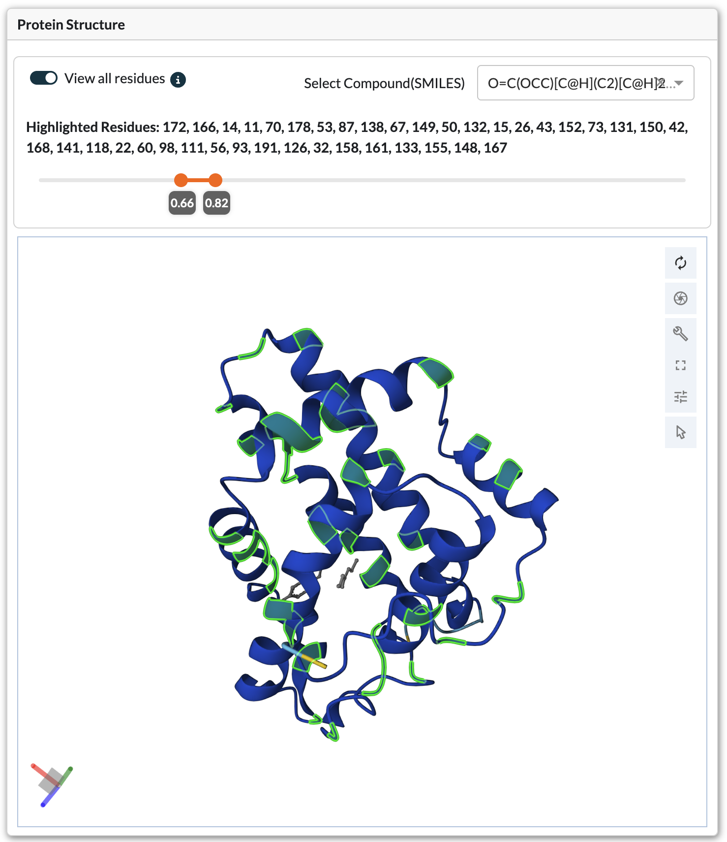
3D protein structure viewer with highlighted mutation positions
Navigation Controls: - Rotate: Left-click and drag - Zoom: Scroll wheel or pinch gesture - Pan: Right-click and drag (or Ctrl + left-click) - Reset View: Click the home icon in viewer controls
Residue Highlighting
Residues can be highlighted in two ways:
Table Selection*: Select a variant row to highlight its mutation positions
View All Residues Mode:
Enable the “View All Residues” toggle switch
Use the Fitness Ratio Slider to set threshold (e.g., 1.5-5.0)
Viewer highlights all residues appearing in variants above threshold
Filter by specific substrate/product using SMILES dropdown
Info text displays which residues are currently highlighted
Top Variants Table
Features:
Displays all variants from the experiment
Rows are color-coded by fitness ratio
Select rows to highlight mutations in the 3D protein viewer
Filter by fitness ratio range using slider controls
Selection:
Single Selection: Click any row to select it
Multi-Selection: Hold Ctrl (Cmd on Mac) and click multiple rows
Filtering and Sorting:
Column Filters: Click the filter icon in column headers
Text Search: Type in filter boxes to search within specific columns
Sorting: Click column headers to toggle ascending/descending sort
Heatmap Visualization
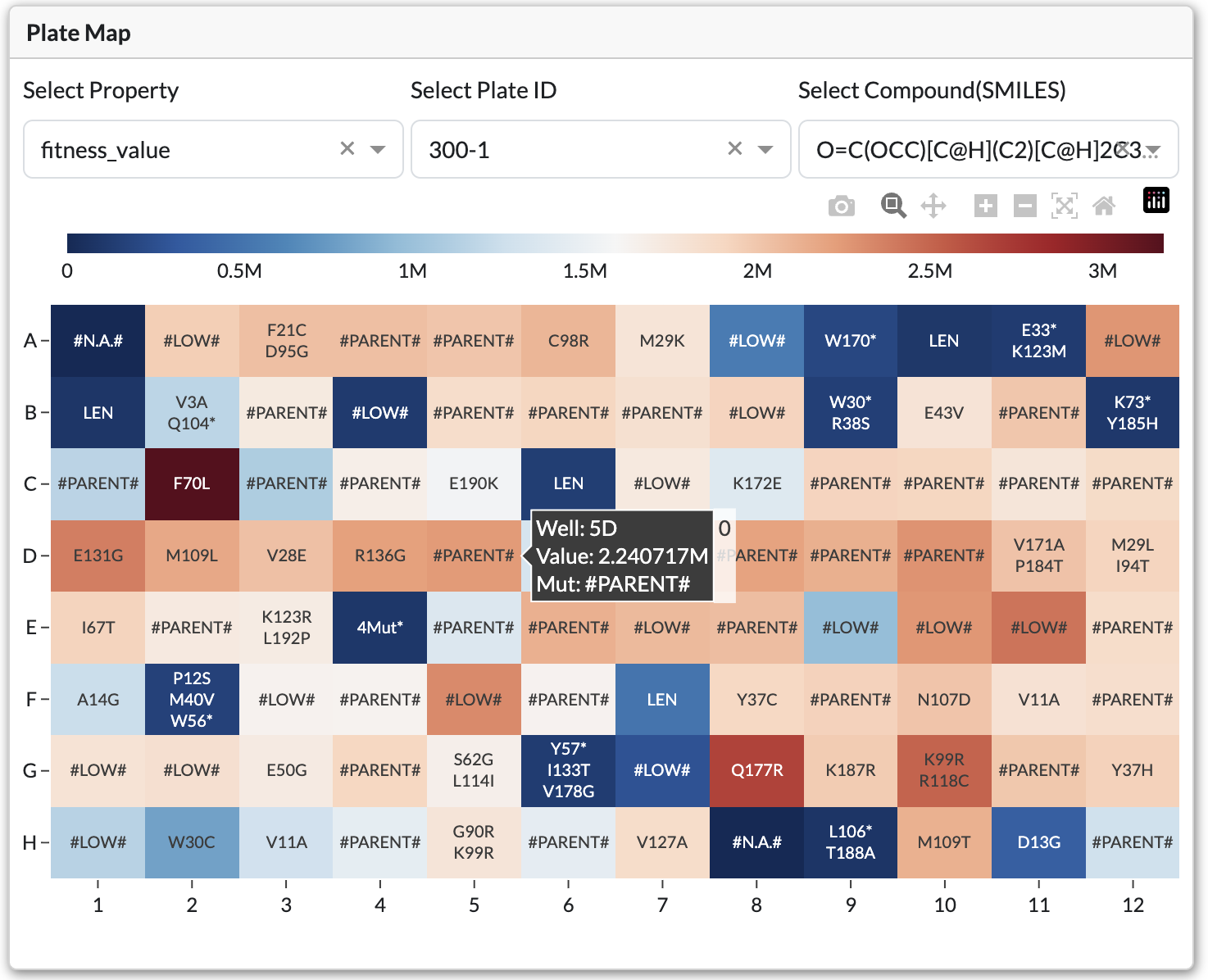
Interactive heatmap showing fitness values color-coded by well position
Visualizes variant data across well plates with color-coded values.
Controls:
Plate Dropdown: Select which plate to view
SMILES Dropdown: Choose substrate/product combination
Property Dropdown: Select visualization property:
Fitness: Shows fitness values
Mean/Median/Std Dev: Statistical summaries across plates
Interactions:
Click individual wells to see detailed variant information
Hover over wells for quick data preview
Retention of Function Curve
Bar chart displaying ranked variants by fitness value
Shows all variants ranked by fitness value. Bars are color-coded by fitness ratio relative to parent.
Controls:
Plate Dropdown: Filter by specific plate
SMILES Dropdown: Filter by substrate/product
Chart Elements:
X-axis: Variant identifier or mutation
Y-axis: Fitness value
Hover: Displays detailed variant information
Single-Site Mutagenesis (SSM) Plot
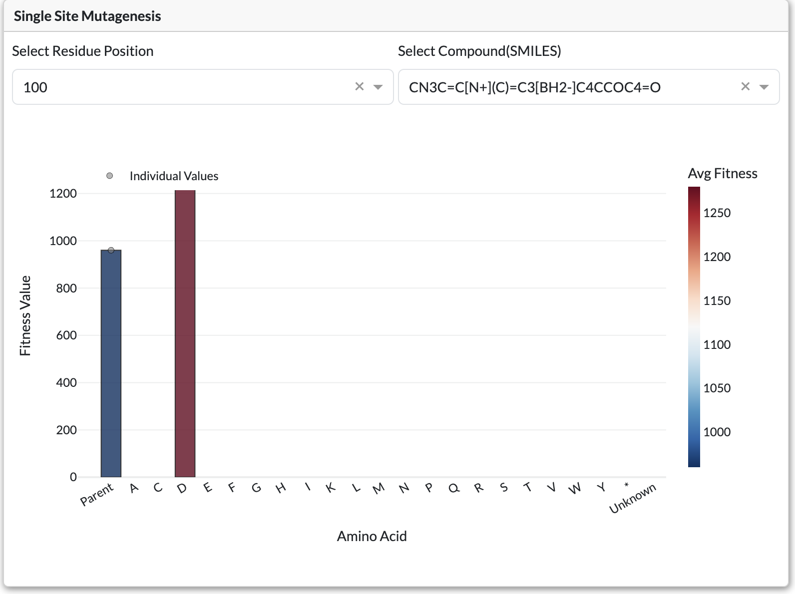
Single-Site Mutagenesis plot displaying fitness values for all amino acid substitutions at a position
Appears for Site Specific experiments instead of retention of function curve. Shows fitness for each amino acid substitution at a selected position.
Controls:
Residue Position Dropdown: Select which position to analyze
SMILES Dropdown: Filter by substrate/product
Chart Elements:
Bars: Fitness value for each amino acid substitution
Dotted Line: Parent sequence fitness (reference)
Hover: Shows amino acid and fitness details
Related Variants Tabs
Find experiments with similar sequences that have variants at specific positions.
Related Variants tab displaying similar experiments with variants at lookup positions.
Setup
Query sequence is auto-filled with current experiment’s parent sequence
Set Alignment Threshold (default 0.8): Minimum sequence similarity (0-1 scale, where 1.0 = 100% match)
Enter Lookup Residues: Comma-separated positions to check (e.g., “100,150,200”)
Click Run to search
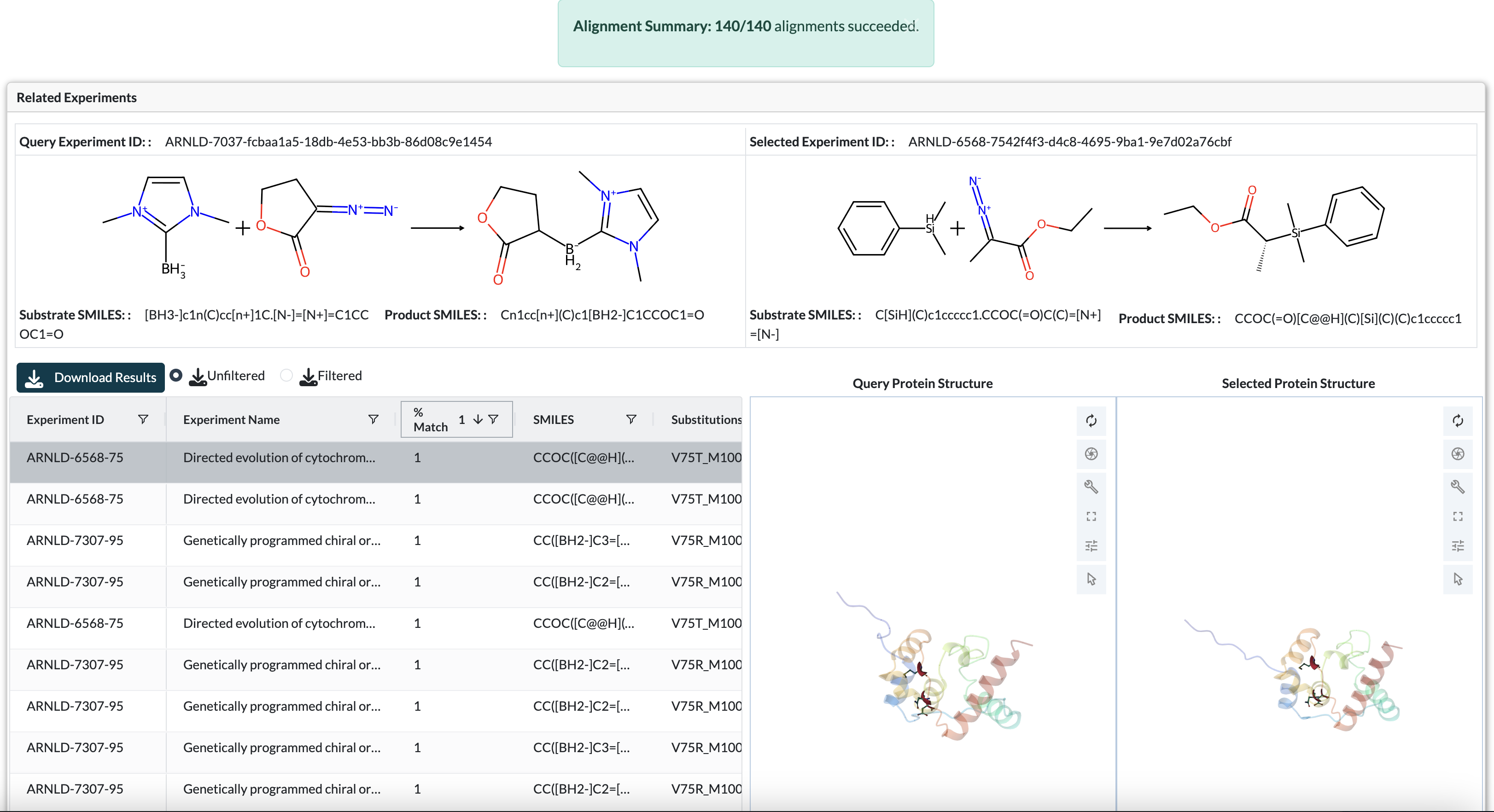
Understanding Results and Comparison View
Table shows experiments with similar parent sequences and with variants at lookup positions
Select a row to compare protein structures side-by-side
Reaction images shows substrate/product for comparison
Left protein structure panel shows current experiment structure with highlighted positions
Right protein structure panel shows selected match structure with highlighted positions
Color Coding:
Red*: Gain-of-function variants
Blue*: Loss-of-function variants
Purple*: Positions that both showed GoF and LoF variants
Sequence Alignment
The Sequence Alignment feature allows you to search across all experiments in the database to find those with similar parent sequences to your query. This is particularly useful for:
Identifying related enzyme variants across different experiments
Finding experiments that may have explored similar sequence space
Comparing gain-of-function and loss-of-function mutations across related proteins
Discovering which residue positions are critical for function across protein families
Overview
The alignment tool uses BLASTP-style pairwise sequence alignment to compare your query sequence against all parent sequences in the database. When matches are found, the system analyzes the variants in those experiments to identify positions that consistently show gain-of-function (GoF) or loss-of-function (LoF) mutations.
Running an Alignment Search
Step 1: Navigate and Enter Query
Navigate to Matching Sequences page from the sidebar
Enter your query protein sequence in the text area:
Must be a valid amino acid sequence (single-letter codes)
Remove any non-sequence letters (e.g., whitespace, numbers, >, <)
Step 2: Configure Search Parameters
Alignment Threshold (0-1 scale):
Sets the minimum sequence identity for matches to be returned, where 1.0 = 100% match
Default: 0.8 is recommended as a starting point
Lower values (0.6-0.7) will find more distantly related sequences
Higher values (0.9-1.0) will only find very similar sequences
Example: 0.8 means at least 80% of aligned positions must be identical
Top N GoF/LoF Positions:
Specifies how many gain-of-function and loss-of-function positions to identify
Default: Top 2 for each category
These positions are ranked by the magnitude of fitness change across variants
Helps focus on the most impactful mutations
Step 3: Execute Search
Click Run Alignment to start the search. The system will:
Align your query against all database parent sequences
Filter results by the alignment threshold
Analyze variants at each position in matching experiments
Identify and rank positions showing gain or loss of function
Understanding the Results
Matched Sequences Table
This table displays all experiments with parent sequences that meet your alignment threshold:
Key Columns:
Experiment ID: Click to navigate to the full experiment page
Alignment Score: Raw alignment score from the pairwise alignment algorithm
Percent Identity: Percentage of aligned positions that are identical matches
Substitutions: Amino acid differences between query and target sequence
Gap Count: Number of insertions/deletions in the alignment
Parent Sequence Length: Length of the matched parent sequence
Interpreting Results:
Higher percent identity indicates more similar sequences
Review substitutions to understand key differences between sequences
Experiments with similar percent identity but different substitutions may have explored different regions of sequence space
Gain-of-Function (GoF) and Loss-of-Function (LoF) Mutations Table
This table aggregates mutation data across all matched experiments to identify critical residue positions:
Understanding GoF Mutations (marked in red):
Positions where mutations consistently lead to increased fitness values
Fitness ratio > 1.0 relative to parent sequence
These positions may represent opportunities for enhancing enzyme activity
Higher fitness values indicate stronger gain-of-function effects
Understanding LoF Mutations (marked in blue):
Positions where mutations consistently lead to decreased fitness values
Fitness ratio < 1.0 relative to parent sequence
These positions may be critical for maintaining protein structure or catalytic function
Lower fitness values indicate stronger loss-of-function effects
Table Columns:
Position: Residue position number in the aligned sequence
Mutation Type: GoF (gain), LoF (loss), or Both (positions showing mixed effects)
Average Fitness Ratio: Mean fitness across all variants at this position
Count: Number of different amino acid substitutions observed at this position
SMILES: Substrate/product combinations where effects were observed
Top Variants: Specific mutations with highest/lowest fitness
Export Options:
Click Export to download the table as CSV for further analysis
Use in downstream analysis, publication figures, or experimental design
Protein Structure Visualization
When you select a row from the Matched Sequences table, the 3D protein structure viewer displays the matched experiment’s structure with color-coded mutation positions:
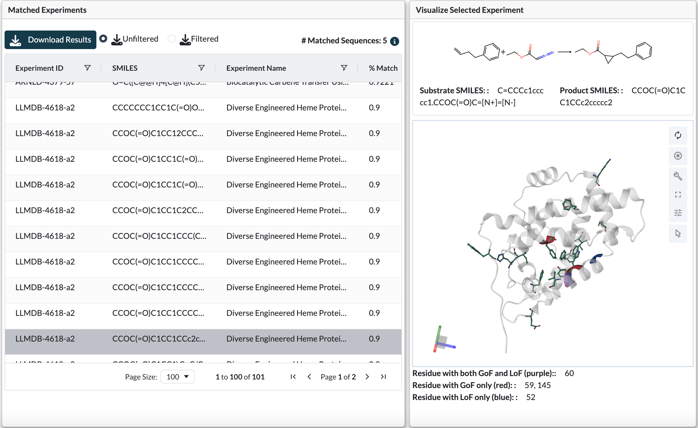
Protein structure viewer displaying gain-of-function (red), loss-of-function (blue), and mixed (purple) mutation positions
Color Coding Scheme:
Red residues: Positions where gain-of-function mutations were observed
Blue residues: Positions where loss-of-function mutations were observed
Purple residues: Positions showing both GoF and LoF mutations
Viewer Interactions:
Rotate, zoom, and pan to examine positions in 3D structural context
Identify whether GoF/LoF positions cluster together (potential active site)
Check if critical positions are on protein surface or buried in core
Look for spatial relationships between different mutation types
Tips for Effective Alignment Searches
Choosing Alignment Threshold:
Start with 0.8 if you’re unsure
Use 0.9-1.0 for finding very closely related variants (same protein family)
Use 0.6-0.8 for finding more distant homologs or related enzyme classes
Lower thresholds will increase search time but may reveal interesting distant relationships
Performance Considerations:
Searches typically complete in seconds to minutes depending on database size
Very long query sequences (>1000 AA) may take longer
Large numbers of matches (>100) may take time to analyze variants